Embeddings

Overview

Large language models (LLMs) do not understand letters or words. To work, LLMs require inputs such as words to be converted into numerical representations that can be computationally processed by the neural network to perform its task. It is these encodings of inputs (e.g., text, documents, images, audio, etc.) into numerical form that we call embeddings. An embedded dataset allows algorithms to quickly search, sort, group information, and more.

LLM chatbot applications such as ChatGPT use the vectors of inputted queries to relate, accelerate and support the generation of its outputs.

For LLMs to achieve semantic understanding, they must be able to correlate the numerical value of words or tokens to one another. For example, the numerical values of the word “dog” and “wolf” should be closer in value than that of the word “airplane”. While it is easy for us to correlate the appearance of the object, there are many other dimensions of relationships between words that must also be accounted for such as semantic meaning, etc.

So, what exactly are these numerical representations? Embeddings are more formally known as vectors, or simply a list of numbers within a matrix separated by commas. For example, below is a fictitious vector for the word “dog”:

dog = [4, 32, 51]

In this example, “dog” is a three-dimensional vector as denoted by the three values (coordinates) separated by commas. The values are used to describe many different attributes of the word. One would expect the vector values of the word “dog” to be closer to the values of “wolf” than the word “apple”.

A simple vector space of three dimensions can be visualized in the graph below:

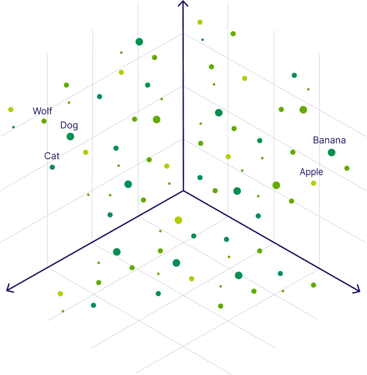
Source: Weaviate.io

The distance between the points can be easily seen and calculated to determine the relationship between the different words.

Because there are so many different attributes, relationships, and contexts between words and sentences, vectors used within LLMs typically consist of over 1,000 dimensions. OpenAI uses a vector space with 1,536 dimensions for each word. Vector embeddings are simply a fancy term for a set of coordinates of a given point in an n-dimensional space used to describe information. A vector embedding model can encode any phrase, paragraph or even an entire document.

While any multi-dimensional vector space over three dimensions is difficult for humans to visualize, computers can efficiently compute the distance between vector spaces to logically understand the relationship or closeness between the values.

In today’s models, pieces of information such as full sentences are encoded within vector databases to determine the meaning of sentence inputs and support the generation of meaningful outputs or answers.

It is important to note that different embedding algorithms will create different embedding vector values for a given input. When using a vector database (a database specifically designed to store and retrieve embedding vectors) in conjunction with a Large Language Model (LLM) such as ChatGPT (i.e. GPT-3.5), the effectiveness of the embeddings stored in the vector database largely depends on how the values align with the embedding algorithm of the LLM. Here’s a breakdown of some key embedding aspects to consider:

Consistency in the Embedding Space: For the most effective use of a vector database alongside an LLM, it’s ideal if the embeddings in the database are generated using the same algorithm or a compatible one as the LLM. This ensures that the embeddings share a consistent semantic space. In other words, similar concepts and contexts are represented by similar vectors, which is crucial for tasks like semantic search, clustering, or similarity assessment.
Transferability of Embeddings: If the embeddings in the vector database are generated using a different model or method, there might be a mismatch in the way semantic information is encoded. This can lead to less effective or inaccurate results when performing operations that rely on vector similarity.
Fine-Tuning and Adaptation: In some cases, one can adapt embeddings from one model to be more compatible with another. This can involve techniques like fine-tuning the LLM on a specific dataset or using transformation techniques to align the embedding spaces of two different models.
Use Case Specificity: The necessity for using the same embedding algorithm depends on the specific use case. For certain applications, like general semantic searches, having embeddings from the same LLM may be crucial. However, for other applications, this might be less critical, and different embedding sources could still provide valuable insights.
Hybrid Approaches: Sometimes, a hybrid approach is used where embeddings from different sources are combined or used in parallel to leverage their unique strengths. This might involve using embeddings from an LLM for textual understanding and embeddings from another source for domain-specific knowledge.

Embedding Use Cases

Many of today’s business applications make use of embeddings:

Google Search uses embeddings to match text to text and text to images
Snapchat uses them to “serve the right ad to the right user at the right time“
Meta (Facebook) uses them for their social search.

Embeddings can also be found in production machine learning systems across a variety of different fields including NLP, recommender systems, and computer vision:

Recommender Systems

A recommender system predicts the preferences and ratings of users for a variety of entities/products. The two most common approaches are collaborative filtering and content-based. Collaborative filtering uses actions to train and form recommendations. Modern collaborative filtering systems almost all use embeddings. The embeddings of recommender systems can be used to support other systems. For example, YouTube’s recommender uses embeddings as inputs to a neural network that predicts watch time.

Semantic Search

Whether it’s a customer support page, a blog, or Google, a search bar should understand the intent and context of a query, not just look at words. Search engines used to be built around TF-IDF, which also creates an embedding from text. This kind of semantic search worked by finding a document embedding that matched closest to the query embedding using the nearest neighbor approach. Today, semantic search utilizes more sophisticated embedding approaches such as BERT.

Computer Vision

In computer vision, embeddings are often used as a way to translate between different contexts. For example, if training a self-driving car, one can transform the image from the car into an embedding and then decide what to do based on that embedded context. By doing so, one can perform transfer learning. One can take a generated image from a game like Grand Theft Auto, turn it into an embedding in the same vector space, and train the driving model without having to feed it tons of expensive, real-world images. Tesla is doing this in practice today.

Vector Databases

Vector databases are databases designed to operationalize the embedding vectors. Vector databases were designed initially utilizing an approach called “One-Hot Encoding”.

One-hot encoding was a common method for representing categorical variables. This unsupervised technique mapped a single category to a vector and generated a binary representation of the specific category. This approach was performed by creating a vector with a dimensional size equal to the number of categories in a given set. As seen in the example below, there are three food categories, equating to a vector space of 3. For each entry in the database, every value is set to 0 except the specific category entry (ID) for that row:

Source: FeatureForm

This approach works by turning a category into a set of continuous variables. Depending on the number of categories, this approach is often inefficient as one will end up with a very large vector of 0s with a single or a handful of 1s. Additionally, since each item is technically equidistant in the vector space, one hot encoding is not able to contextualize the similarity or obtain a semantic relationship of category values.

This means that the words “dog” and “wolf” are no closer together than “dog” and “airplane”. As a result, there is no way of evaluating the relationship between two entities without performing additional inefficient relationship mappings and calculations.

Vector database design evolved from one-hot encodings to not only store and retrieve multi-dimensional vector values, but to also perform vector embedding calculations to support AI models.

Creating Embeddings

A common way to create an embedding requires us to first set up a supervised machine-learning problem. As a side-effect, training that model encodes categories into embedding vectors. For example, one can set up a model that predicts the next movie a user will watch based on what they are watching now. An embedding model will factorize the input into a vector and that vector will be used to predict the next movie. This means that similar vectors are movies that are commonly watched after similar movies. This makes for a great representation to be used for personalization. So even though one is solving a supervised problem, often called the surrogate problem, the actual creation of embeddings is an unsupervised process.

Defining a surrogate problem is an art, and dramatically affects the behavior of the embeddings. For example, YouTube’s recommender team realized that using the “predict the next video a user is going to click on” resulted in clickbait becoming rampantly recommended. They moved to “predict the next video and how long they are going to watch it” as a surrogate problem and achieved far better results.

Embedding Models

There are many different types of embedding models:

Principal Component Analysis (PCA)

One method for generating embeddings is called Principal Component Analysis (PCA). PCA reduces the dimensionality of an entity by compressing variables into a smaller subset. This allows the model to behave more effectively but makes variables more difficult to interpret, and generally leads to a loss of information. A popular implementation of PCA is a technique called SVD.

SVD

Singular Value Decomposition, also known as SVD, is a dimensionality reduction technique. SVD reduces the quantity of data set features from N-dimensions to K-dimensions via matrix factorization. For example, let’s represent a user’s video ratings as a matrix of size (Number of users) x (Number of Items) where the value of each cell is the rating that a user gave that item. A number, k, is selected as the embedding vector size. SVD is used to split the table into two matrices. One will be (Number of users) x k and the other will be k x (Number of items).

In the resulting matrices, if the user vector is multiplied by the item vector, one should obtain the predicted user rating. If both matrices are multiplied, it would result in the original matrix, but densely filled with all of the predicted ratings. It follows that two items that have similar vectors result in a similar rating from the same user. The result is that embeddings are created for users and items.

Source: FeatureForm

Word2Vec

Word2vec was a novel approach that utilized neural networks to establish the vector values of words. In 2010, Tomáš Mikolov applied a simple recurrent neural network with a single hidden layer to determine the values. Word2vec was patented and published in 2013 by a team of researchers led by Mikolov. By 2022, the Word2vec approach was described as “dated”, with transformer models being regarded as the state of the art in NLP.

To generate embeddings using the Word2Vec approach, words are encoded into one-hot vectors and fed into a hidden layer that generates hidden weights. Those hidden weights are then used to predict other nearby words. Although these hidden weights are used for training, Word2Vec will not use them for the task it was trained on. Instead, the hidden weights are returned as embeddings and the model is tossed out.

Source: FeatureForm

Words that are found in similar contexts will have similar embeddings. Beyond that, embeddings can be used to form analogies. For example, the vector from king to man is very similar to the one from queen to woman.

One problem with Word2Vec is that single words have one vector mapping. This means that all semantic uses for a word are combined into one representation. For example, the word “play” in “I’m going to see a play” and “I want to play” will have the same embedding, without the ability to distinguish context.

Source: FeatureForm

BERT

Bidirectional Encoder Representations of Transformers, also known as BERT, is a pre-trained model that solves Word2Vec’s context problems. BERT was introduced in October 2018 by researchers at Google. A 2020 literature survey concluded that “in a little over a year, BERT has become a ubiquitous baseline in Natural Language Processing (NLP) experiments counting over 150 research publications analyzing and improving the model.”

BERT is trained in two steps. First, it is trained across a huge corpus of data like Wikipedia to generate similar embeddings as Word2Vec. The end-user performs the second training step. They train on a corpus of data that fits their context well, for example, medical literature. BERT will be fine-tuned for that specific use case. Also, to create a word embedding, BERT takes into account the context of the word. That means that the word “play” in “I’m going to see a play” and “I want to play” will correctly have different embeddings. BERT has become the go-to transformer model for generating text embeddings. Google uses BERT on a large percentage of its queries.

Embedding Operations

The vector values of embeddings can be used to perform different operations including:

Averaging

Using something like Word2Vec, one can end up with an embedding for each word, but one often needs an embedding for a full sentence. Similarly, in recommender systems, one may know the items a user clicked on recently, but the user embedding may not have been retrained in days. In these situations, we one average embeddings to create higher-level embeddings. In the sentence example, one can create a sentence embedding by averaging each of the word embeddings. In the recommender system, one can create a user embedding by averaging the last N items they clicked.

Subtraction/Addition

Word embeddings can encode analogies via vector differences. Adding and subtracting vectors can be used for a variety of tasks. For example, one can find the average difference between a coat from a cheap brand and a luxury brand. The delta can be stored and used to recommend a luxury item that’s similar to the current item that a user is looking at. The difference between a coke and a diet coke can be determined and applied to other drinks, even to those drinks that don’t have diet equivalents, to find the closest thing to a diet version.

Nearest Neighbor

Nearest neighbor (NN) is often the most useful embedding operation. This operation finds things that are similar to the current embedding. In recommender systems, one can create a user embedding and find items that are most relevant to them. In a search engine, one can find a document that is most similar to a search query. Despite its utility, nearest neighbor operations are computationally expensive. In most cases when nearest neighbors are required, an approximation would suffice. Approximate nearest neighbor (ANN) algorithms are commonly used and typically reduce the computational requirements and associated cost.

Implementations of Approximate Nearest Neighbor (ANN)

There are many different algorithms to efficiently find approximate nearest neighbors, and many implementations of each of them. Below are a few of the most common ANN algorithms:

Spotify’s Annoy

In Spotify’s ANN implementation (Annoy), the embeddings are turned into a forest of trees. Each tree is built using random projections. At every intermediate node in the tree, a random hyperplane is chosen, which divides the space into two subspaces. This hyperplane is chosen by sampling two points from the subset and taking the hyperplane equidistant from them. This is performed k times to generate a forest. Lookups are done via in-order traversal of the nearest tree. Annoy’s approach allows the index to be split into multiple static files, the index can be mapped in memory, and the number of trees can be tweaked to change speed and accuracy.

Here’s how Annoy breaks down the embeddings into an index of multiple trees via random projections:

Source: FeatureForm

Locality Sensitive Hashing (LSH)

Locality Sensitive Hashing (LSH) employs a hash table and stores nearby points in their respective buckets. LSH keeps points with large distances in separate buckets. To retrieve the nearest neighbor, the point in question is hashed, a lookup is performed, and the closest query point is returned.

Facebook’s FAISS and Hierarchical Navigable Small World Graphs (HNSW)

Facebook’s ANN implementation, FAISS, uses Hierarchical Navigable Small World Graphs (HNSW). HNSW typically performs well in accuracy and recall. It utilizes a hierarchical graph to create an average path towards certain areas. This graph has a hierarchical, transitive structure with a small average distance between nodes. HNSW traverses the graph and finds the closest adjacent node in each iteration and keeps track of the “best” neighbors found.

HNSW works by creating a hierarchical index to allow for faster nearest neighbor lookup.

Source: FeatureForm

Operationalizing Embeddings

Moving embeddings out of labs and into real world systems surfaced real gaps in current data infrastructure capabilities. For example, traditional databases and caches don’t support operations like nearest neighbor lookups. Specialized approximate nearest neighbor indices lack durable storage and other features required for full production use. MLOps systems lack dedicated methods to manage versioning, access, and training for embeddings. Modern ML systems need an embedding store: a database built from the ground up around the machine learning workflow with embeddings.

Additionally, promoting embeddings into production isn’t easy. The most common ways embeddings operationalized today are via Redis, Postgres, and S3 + Annoy/FAISS:

Redis

Redis is a super-fast in-memory object-store. It makes storing and retrieving embeddings by key very fast. However, it does not maintain any native embedding operations. It can’t perform nearest-neighbor lookups and it can’t add or average vectors. All of these operations must be performed on the model service. It also does not fit cleanly in a typical MLOps workflow. Redis does not support versioning, rolling back, or maintaining immutability. When training, the Redis client does not automatically cache embeddings which can cause unnecessary pressures and increase costs. Lastly, Redis also does not support partitioning embeddings and creating sub-indices.

Postgres

Postgres is far more versatile, but far slower than Redis. Via plugins, Postgres can perform some of the vector operations manually. However, Postgres does not maintain a nearest neighbor index. Also, Postgres lookups that are part of a model’s critical path may add too much latency. Finally, Postgres does not have a great way to cache embeddings on the client when training and can result in very slow training times.

S3 Files + Annoy/FAISS

Annoy or FAISS are often used to operationalize embeddings when nearest-neighbor lookups are required. Both systems build indices of embeddings for approximate nearest neighbor operations, but they do not handle durable storage or other vector operations. Alone, they only solve one problem. Typically, companies will store their embeddings in S3 or a similar object storage service to fill in the rest of the gaps. They will load the embeddings and create the ANN index directly on the model when required. Updating embeddings becomes tough, and the system typically ends up with a lot of ad-hoc rules to manage versioning and rollbacks. FAISS and Annoy are great, but they require a full embedding store built around them.

The Embedding Hub

Machine learning systems that use embeddings require data infrastructure that:

Stores their embeddings durably and with high availability
Allows for approximate nearest neighbor operations
Enables other operations like partitioning, sub-indices, and averaging
Manages versioning, access control, and rollbacks painlessly

A few companies like Pinterest have built their own in-house embedding infrastructure, but the gap remains. Some startups are working to build proprietary systems, and some database companies are trying to add nearest neighbors capabilities to their existing product offerings.

Additionally, gaps are present in the open-source world. Featureform is one organization that has made its Embedding Hub available on Github.